Introduction
Heyo there! with a lot of buzz going around machine learning and deep learning, I wanted to try out using a RNN (Recurrent neural network) model to see how well it can predict the closing price of a cryptocurrency. Machine learning models have gotten really good at modeling real world data, so I wanted to see how well it can do with predicting crypto movements after training it with historical data.
Machine learning models are evaluated based on many parameters like accuracy, precision and recall but the most importantly, how well can it do a task as an experienced human would perform. There was a interesting study that showed how monkeys can outperform fund managers when picking stocks over a one year period (while that might not apply to crypto) it’s probably fair to say that we cannot reliably predict the closing price given just the historical data.
Deep learning models have been applied to a lot of really difficult tasks like image classification, speech recognition, and even self driving cars. Each model is trained and retrained using a lot of data and of different types for more accurate results. For a sequence of data, RNN models are a good starting point since the output of the next node in a layer depends on the output of the previous ones. This helps it set weights and biases for the current layer and fine tunes it based on the training data provided. Since historical data is usually sequenced in time so it would be helpful to use it for trying to predict a value in the future given a window of 30-60 days.
There’s also a tutorial video on using Google Colab to build RNN models for predicting closing prices that goes over more details on why they’re needed and how to hook them up all together.
Requirements
For setting up, you need jupyter notebook installed along with Tensorflow and scikit-learn these libraries help you use the models, scalers and any other plotting utils that might be needed. After installing all the packages we can start with setting up the notebook.
Setting up notebook
First lets import all the packages we might need.
import math
import numpy as np
import pandas as pd
from sklearn.preprocessing import MinMaxScaler
from keras.models import Sequential
from keras.layers import Dense, LSTM
import matplotlib.pyplot as plt
import matplotlib.dates as mdates
import requests
from io import StringIO
Next before we start defining the model, we want to setup parameters that can be used to train the model.
Using Hyperparameters for training the model
Next, we need to setup model parameters or hyperparameters that allow you to fine tune the model and use different behavior when training it. Based on the dataset, some parameters like batch size, epochs have huge impact on how well the model fits to the training data. If it overfits, the training sample it might not be general enough to predict values outside of the training set, or if it’s underfits the training sample it wouldn’t be very accurate in predictions for training and test (validation) datasets.
### Model parameters
num_of_days = 200
batch_size = 1
epochs = 1
btc_symbol = 'BTC-USD'
Kaggle had a great article on overfitting and underfitting and how to identify if the model is behaving in a weird way.
Fetching the data
Now we can fetch the data needed for training and validating the model.
base_url = 'https://query1.finance.yahoo.com/v7/finance/download'
user_agent_headers = {
    'User-Agent': 'Mozilla/5.0 (Macintosh; Intel Mac OS X 10_10_1) AppleWebKit/537.36 (KHTML, like Gecko) Chrome/39.0.2171.95 Safari/537.36'
}
params = {
    'interval': '1d',
    'events': 'history',
    'range': '5y'
}
response = requests.get(f'{base_url}/{btc_symbol}', params=params, headers=user_agent_headers)

# Historical data
data = StringIO(response.text)

data = pd.read_csv(data, index_col='Date').dropna()
data['Date'] = data.index
data
Once we have the information needed let’s quickly double check if the data is in the right format.
data.shape # (1822, 7) Number of records (1822), attributes like open, high, low, close, volume, etc (7).
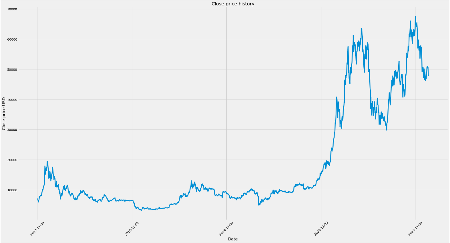
Awesome, now lets plot it and see what it looks like.
plt.style.use('fivethirtyeight')
# Plot closing price of ticker
plt.figure(figsize=(30, 16))
plt.title('Close price history')
plt.plot(data.index, data['Close'])
plt.xlabel('Date', fontsize=18)
plt.ylabel('Close price USD', fontsize=18)
plt.gca().xaxis.set_major_locator(mdates.YearLocator())
plt.xticks(rotation=45)
plt.autoscale()
plt.show()

Split data into training and validation sets
Cool now let’s split the data up in training and validation datasets. For this we will use 80% for training and 20% for validation.
# Prepare data
dataset = data.filter(['Close'])
print(dataset)
# convert to numpy array
dataset = dataset.values

training_data_len = math.ceil(len(dataset) * 0.8)
print(dataset)
print(training_data_len)
Date        Close
2016-09-06    610.435974
2016-09-07    614.544006
2016-09-08    626.315979
2016-09-09    622.861023
2016-09-10    623.508972
...                  ...
2021-09-01  48847.027344
2021-09-02  49327.722656
2021-09-03  50025.375000
2021-09-04  49944.625000
2021-09-06  51590.382813

[1822 rows x 1 columns]
[[  610.435974]
 [  614.544006]
 [  626.315979]
 ...
 [50025.375   ]
 [49944.625   ]
 [51590.382813]]
1458
Transform training data
Before we split the data, we would need to scale it appropriately, if some attributes have a higher value than others it could skew the models towards higher value attributes. Example, if the price change is near 1-4% but the volume traded might be in thousand to millions, it could skew the model to prefer volume vs price change.
# Setup scaler
scaler = MinMaxScaler(feature_range=(0, 1))
scaled_data = scaler.fit_transform(dataset)

scaled_data
array([[2.24743896e-04],
       [2.90046988e-04],
       [4.77179473e-04],
       ...,
       [7.85746452e-01],
       [7.84462814e-01],
       [8.10624508e-01]])
The MinMaxScaler fits all the values between 0 and 1, so the highest value gets assigned 1 and the lowest gets assigned 0 and all other values in between get a value between 0 and 1.
Let’s setup the training data for the model.
# Setup training data for model
train_data = scaled_data[0:training_data_len, :]
# Split data in x_train and y_train
x_train = []
y_train = []

for i in range(num_of_days, len(train_data)):
    x_train.append(train_data[i-num_of_days:i, 0])
    y_train.append(train_data[i, 0])
In the training split x_train is what is used as the initial input to the model so 0-199 days historical data is used to predict the y_train value of day 200, and 1-200 is used to predict the value of day 201. You can play around with the number of days to see which one works better.
Sweet, now let’s get the training data all prepped up for the model to use.
# convert x_train and y_train to numpy arrays
x_train, y_train = np.array(x_train), np.array(y_train)
# Reshape data
x_train = np.reshape(x_train, (x_train.shape[0], x_train.shape[1], 1))
x_train.shape
(1258, 200, 1)
Building the model
For building the RNN model layers we’re using the an input LSTM (Long short-term memory) a hidden LSTM, and dense layers for getting the outputs from previous layers.
# Build LSTM model
model = Sequential()
model.add(LSTM(50, return_sequences=True, input_shape=(x_train.shape[1], 1)))
model.add(LSTM(50, return_sequences=False))
model.add(Dense(25))
model.add(Dense(1))
After it’s setup, we can now train the model using the training set.
# Train the model
model.fit(x_train, y_train, batch_size=batch_size, epochs=epochs)
1258/1258 [==============================] - 60s 47ms/step - loss: 6.6969e-04
<tensorflow.python.keras.callbacks.History at 0x7f0f13f0c1c0>
Validation predictions
The loss function should gradually decrease as the model learns from the training set. Now we can test the predictions from the validation set and how well it predicted values for the last 200 days.
# Create test data sets
test_data = scaled_data[training_data_len - num_of_days: , :]
# Create scaled x_test, y_test
x_test = []
y_test = dataset[training_data_len: , :]
for i in range(num_of_days, len(test_data)):
    x_test.append(test_data[i-num_of_days: i, 0])
The y_test is not the actual closing price but a scaled result, so we would need to scale it back to the original values after the model outputs a predicted value.
Let’s set up a test data set for the model.
# Convert test data to numpy array
x_test = np.array(x_test)
# Reshape data
x_test = np.reshape(x_test, (x_test.shape[0], x_test.shape[1], 1))
x_test.shape
(364, 200, 1)
And finally getting back the predictions from the model on the validation set.
# get model predictions
predictions = model.predict(x_test)
predictions = scaler.inverse_transform(predictions)
Sweet, now we should calculate the total loss or mean squared error from the actual values.
# Calculate root mean squared error
rmse = np.sqrt(np.mean(predictions - y_test) ** 2)
rmse
3078.505888980426
Plotting results
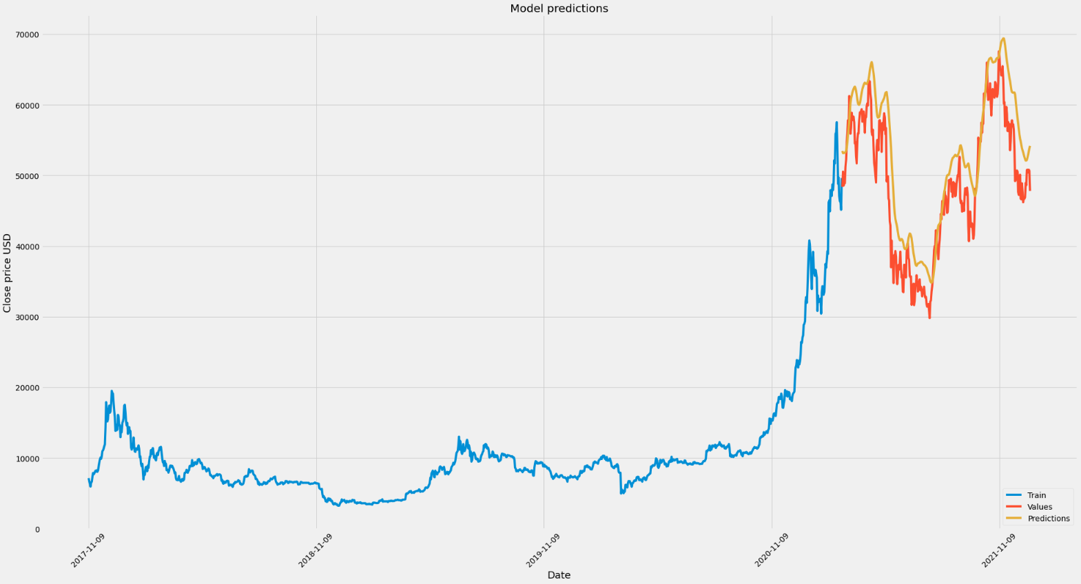
Ideally if the model predicted the exact value as expected the total loss would be 0. We can now plot the predicted values alongside the actual values of closing price for BTC.
# Plot the predicted values
train = data[:training_data_len]
valid = data[training_data_len:]
valid['Predictions'] = predictions

plt.figure(figsize=(16, 8))
plt.title('Model')
plt.xlabel('Date', fontsize=18)
plt.ylabel('Close price USD', fontsize=18)
plt.plot(train['Close'])
plt.plot(valid[['Close', 'Predictions']])
plt.legend(['Train', 'Values', 'Predictions'], loc='lower right')
plt.show()

Conclusion
Not too far off for a really volatile crypto like BTC, but did find it interesting that initially the predicted values were very close to the actual values. But the errors started to compound as the model started to learn from the predicted values. Pretty impressive for using a simple RNN model from Tensorflow and Keras. It might be better to use more inputs like volume and other technical indicators that could maybe reduce errors in predicted values, but really cool to see in action.
That’s all folks, hope this was helpful!
Join the email list and get notified about new content
Be the first to receive latest content with the ability to opt-out at
anytime.
We promise to not spam your inbox or share your email with any third
parties.


